Linear Programming Excel Case Study – Logistics Optimization
Real-World Excel Logistics Optimization Model: Fleet Delivery Example
In this second case study, we turn our attention to the logistics sector—a field where cost efficiency and time management are critical. This linear programming Excel case study focuses on a delivery company tasked with meeting customer demands at five distribution points using three trucks with different capacities and associated fuel costs.
Objective
To minimize total delivery cost while satisfying customer demands and adhering to truck capacity constraints. A well-built linear programming Excel model can help us reach this goal efficiently.
Key Data for the Linear Programming Excel Logistics Model
Truck Capacities
| Truck | Capacity (Units) |
| T1 | 100 |
| T2 | 80 |
| T3 | 60 |
Warehouse Demand
| Warehouse | Required Units |
| W1 | 50 |
| W2 | 40 |
| W3 | 60 |
| W4 | 30 |
| W5 | 60 |
Fuel Cost Matrix (Cost per Unit Delivered)
| W1 | W2 | W3 | W4 | W5 | |
| T1 | 4 | 6 | 5 | 8 | 6 |
| T2 | 5 | 4 | 3 | 7 | 5 |
| T3 | 6 | 5 | 4 | 6 | 4 |
Building the Linear Programming Model in Excel for Logistics Optimization
o make this easier, you can download and explore the actual Excel file used in this case study. It contains:
- Input tables for trucks, warehouses, and fuel costs,
- Predefined decision variable layout,
- Solver configuration ready to test.
👉 Download the Logistics LP Excel Template (Logistics LP)
Decision Variables
Let x_ij be the number of units delivered from truck i to warehouse j. There are 15 such variables (3 trucks × 5 warehouses) in this logistics linear programming Excel case study.
Objective Function
Minimize:
Total Cost = Σ(cost_ij * x_ij)In Excel: =SUMPRODUCT(CostRange, VariableRange)
Constraints
- Each warehouse must receive the exact amount of demand
- Each truck cannot exceed its capacity
- All x_ij values must be ≥ 0
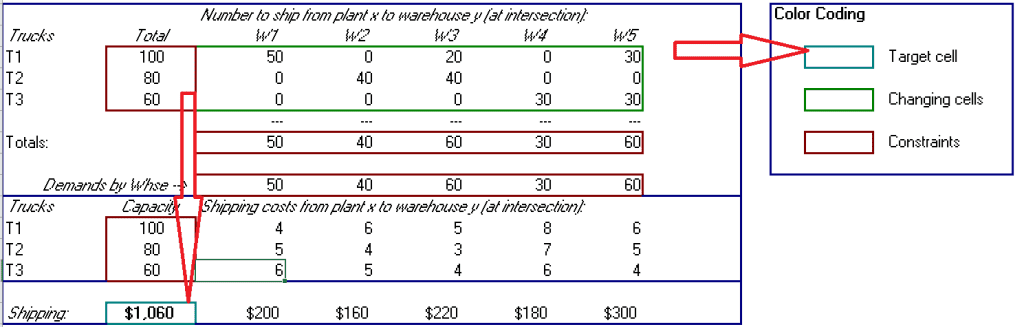
Configuring Excel Solver for Linear Programming in Logistics
- Objective: Minimize total delivery cost (target cell)
- Changing Cells: All x_ij variables
- Constraints:
- Row sums (truck capacity) ≤ respective truck limit
- Column sums (warehouse demand) = required units
- x_ij ≥ 0
- Solving Method: Simplex LP
Click Solve. Solver will generate the optimal distribution plan for this logistics optimization model in Excel in logistics.
Example Output: Optimized Delivery Plan
| From / To | W1 | W2 | W3 | W4 | W5 | Total |
| T1 | 40 | 30 | 30 | 0 | 0 | 100 |
| T2 | 10 | 10 | 30 | 30 | 0 | 80 |
| T3 | 0 | 0 | 0 | 0 | 60 | 60 |
Total Cost: $950. All warehouse demands are met. Truck capacities are fully utilized.
Business Insights from the Programming Excel Logistics Case Study
- Cost Efficiency: Fuel expenses reduced through optimized routing
- Capacity Utilization: No truck exceeded capacity; each was maximized based on cost effectiveness
- Operational Clarity: Managers gain clear visibility into fleet efficiency and route allocation
This logistics optimization model in Excel demonstrates how companies can save thousands through intelligent logistics planning.
What’s Next: Financial Portfolio Optimization with Linear Programming in Excel
In the upcoming third part of this series, we’ll shift focus from logistics to financial strategy. Using the power of linear programming in Excel, we’ll demonstrate how to:
- Construct a diversified investment portfolio,
- Balance expected return with risk exposure,
- Apply Solver to enforce constraints like asset limits, risk thresholds, and diversification rules.
Stay tuned for Part Three: Linear Programming Excel Case Study – Financial Portfolio Optimization, where you’ll learn how to bring precision to your investment planning.